The SAT (Scholastic Aptitude Test) is a standardized test widely used for college admissions in the United States. The test is divided into 3 sections, each of which has a total score of 800. High schools are often ranked by their average SAT scores, and high SAT scores are considered a sign of how good a school district is.
This project utilizes different datasets taken from the NYC OpenData initiative. The main idea here was to combine data from multiple associated data sources and perform exploratory data analysis on it to understand:
- Are schools differentiated by SAT scores?
- The schools which are doing best and the ones which are doing worse, what are the key differentiating factors between these schools?
- Do demographics really play a role in SAT scores? If yes, then how and which demographic categories are doing better than others
Data pull and cleaning
For purpose of this analysis, we will be taking multiple open-source data sets available, perform some cleaning, and consolidate them into one dataset having one row per school, which would then allow us to do the rest of Exploratory Data Analysis pretty easily. As I would be using the NYC OpenData APIs to pull in the data, I have added the links to APIs for downloading the data directly into pandas dataframes.
Before we start with the datasets, I would like to take a moment and explain how the data hierarchy works in these datasets. I did some research and found out that New York is divided into districts (denoted by numbers like 01,02, etc.), which are then further divided into boroughs, which then have schools. Thus, each school is identified by its DBN (District Borough Number) which looks something like “01M015”.
The datasets that we would be using in this project are:
- Sat Scores - SAT Scores by sections for each school. Download JSON here
- Enrollment - Average attendance & Number of students enrolled at a district level. Download JSON here
- High Schools - A plethora of details about every school such as location, address, website, etc. Download JSON here
- Class Size - Details about school class sizes & education programs. Download JSON here
- Advanced Placement - Summary of students taking advanced placement exams by school. Download JSON here
- Graduation - Graduation related stats for each school by cohorts. Download JSON here
- Demographics - Student demographics information for each school. Download JSON here
- Districts - District coordinates and shape polygons. You will need to download this data in GeoJSON format in order to use it for plotting. Download them from here
- Math test results - Math test results for every school. Download JSON here
- Survey Results - Survey responses of students, teachers, and parents for each school providing overview of their perception of school quality. This is not available through APIs and has to be downloaded from here
Having gotten enough context, let’s get started with this project!!
First, we will import the required libraries using the below code:
#Importing all relevant libraries
import numpy as np
import pandas as pd
import os
import folium # For plotting chloropleth charts
from folium import plugins
import pygeoj # For reading in geoJSON District map file
Now, let’s read in all the different datasets that I described above:
#Using Department of Education APIs to read in all relevant data
sat_results = pd.read_json("https://data.cityofnewyork.us/resource/f9bf-2cp4.json")
enrollment = pd.read_json("https://data.cityofnewyork.us/resource/7z8d-msnt.json")
high_schools = pd.read_json("https://data.cityofnewyork.us/resource/n3p6-zve2.json")
class_size = pd.read_json("https://data.cityofnewyork.us/resource/urz7-pzb3.json")
ap2010 = pd.read_json("https://data.cityofnewyork.us/resource/itfs-ms3e.json")
graduation = pd.read_json("https://data.cityofnewyork.us/resource/vh2h-md7a.json")
demographics = pd.read_json("https://data.cityofnewyork.us/resource/ihfw-zy9j.json")
math_results = pd.read_json("https://data.cityofnewyork.us/resource/jufi-gzgp.json")
survey_1 = pd.read_csv("masterfile11_gened_final.txt",delimiter='\t',encoding='windows-1252')
survey_2 = pd.read_csv("masterfile11_d75_final.txt",delimiter='\t',encoding='windows-1252')
Having the data in place, its always good to check samples for each data set to understand it better
#Browsing the datasets one by one
sat_results.head()
| dbn | num_of_sat_test_takers | sat_critical_reading_avg_score | sat_math_avg_score | sat_writing_avg_score | school_name | |
|---|---|---|---|---|---|---|
| 0 | 01M292 | 29 | 355 | 404 | 363 | HENRY STREET SCHOOL FOR INTERNATIONAL STUDIES |
| 1 | 01M448 | 91 | 383 | 423 | 366 | UNIVERSITY NEIGHBORHOOD HIGH SCHOOL |
| 2 | 01M450 | 70 | 377 | 402 | 370 | EAST SIDE COMMUNITY SCHOOL |
| 3 | 01M458 | 7 | 414 | 401 | 359 | FORSYTH SATELLITE ACADEMY |
| 4 | 01M509 | 44 | 390 | 433 | 384 | MARTA VALLE HIGH SCHOOL |
enrollment.head()
| district | ytd_attendance_avg_ | ytd_enrollment_avg_ | |
|---|---|---|---|
| 0 | DISTRICT 01 | 91.18 | 12367 |
| 1 | DISTRICT 02 | 89.01 | 60823 |
| 2 | DISTRICT 03 | 89.28 | 21962 |
| 3 | DISTRICT 04 | 91.13 | 14252 |
| 4 | DISTRICT 05 | 89.08 | 13170 |
high_schools.head()
| :@computed_region_92fq_4b7q | :@computed_region_efsh_h5xi | :@computed_region_f5dn_yrer | :@computed_region_sbqj_enih | :@computed_region_yeji_bk3q | addtl_info1 | addtl_info2 | advancedplacement_courses | bbl | bin | ... | school_name | school_sports | school_type | se_services | start_time | state_code | subway | total_students | website | zip | |
|---|---|---|---|---|---|---|---|---|---|---|---|---|---|---|---|---|---|---|---|---|---|
| 0 | 47 | 20529.0 | 51 | 59 | 3 | Uniform Required: plain white collared shirt, ... | Extended Day Program, Student Summer Orientati... | Calculus AB, English Language and Composition,... | 4.157360e+09 | 4300730.0 | ... | Frederick Douglass Academy VI High School | Step Team, Modern Dance, Hip Hop Dance | NaN | This school will provide students with disabil... | 2020-04-28 07:45:00 | NY | A to Beach 25th St-Wavecrest | 412.0 | http://schools.nyc.gov/schoolportals/27/Q260 | 11691 |
| 1 | 45 | 17616.0 | 21 | 35 | 2 | Our school requires completion of a Common Cor... | NaN | NaN | 3.068830e+09 | 3186454.0 | ... | Life Academy High School for Film and Music | NaN | NaN | This school will provide students with disabil... | 2020-04-28 08:15:00 | NY | D to 25th Ave ; N to Ave U ; N to Gravesend - ... | 260.0 | http://schools.nyc.gov/schoolportals/21/K559 | 11214 |
| 2 | 49 | 18181.0 | 69 | 52 | 2 | Dress Code Required: solid white shirt/blouse,... | Student Summer Orientation, Weekend Program of... | English Language and Composition, United State... | 3.016160e+09 | 3393805.0 | ... | Frederick Douglass Academy IV Secondary School | Basketball Team | NaN | This school will provide students with disabil... | 2020-04-28 08:00:00 | NY | J to Kosciusko St ; M, Z to Myrtle Ave | 155.0 | http://schools.nyc.gov/schoolportals/16/K393 | 11221 |
| 3 | 31 | 11611.0 | 58 | 26 | 5 | All students are individually programmed (base... | Extended Day Program | Art History, English Language and Composition,... | 2.036040e+09 | 2022205.0 | ... | Pablo Neruda Academy | Baseball, Basketball, Flag Football, Soccer, S... | NaN | This school will provide students with disabil... | 2020-04-28 08:00:00 | NY | N/A | 335.0 | www.pablonerudaacademy.org | 10473 |
| 4 | 19 | 12420.0 | 20 | 12 | 4 | Chancellor’s Arts Endorsed Diploma | NaN | Art History, Biology, Calculus AB, Calculus BC... | 1.011560e+09 | 1030341.0 | ... | Fiorello H. LaGuardia High School of Music & A... | NaN | Specialized School | This school will provide students with disabil... | 2020-04-28 08:00:00 | NY | 1 to 66th St - Lincoln Center ; 2, 3 to 72nd S... | 2730.0 | www.laguardiahs.org | 10023 |
5 rows × 69 columns
class_size.head()
| average_class_size | borough | core_course_ms_core_and_9_12_only_ | core_subject_ms_core_and_9_12_only_ | csd | data_source | grade_ | number_of_sections | number_of_students_seats_filled | program_type | school_code | school_name | schoolwide_pupil_teacher_ratio | service_category_k_9_only_ | size_of_largest_class | size_of_smallest_class | |
|---|---|---|---|---|---|---|---|---|---|---|---|---|---|---|---|---|
| 0 | 19.0 | M | - | - | 1 | ATS | 0K | 1.0 | 19.0 | GEN ED | M015 | P.S. 015 Roberto Clemente | NaN | - | 19.0 | 19.0 |
| 1 | 21.0 | M | - | - | 1 | ATS | 0K | 1.0 | 21.0 | CTT | M015 | P.S. 015 Roberto Clemente | NaN | - | 21.0 | 21.0 |
| 2 | 17.0 | M | - | - | 1 | ATS | 01 | 1.0 | 17.0 | GEN ED | M015 | P.S. 015 Roberto Clemente | NaN | - | 17.0 | 17.0 |
| 3 | 17.0 | M | - | - | 1 | ATS | 01 | 1.0 | 17.0 | CTT | M015 | P.S. 015 Roberto Clemente | NaN | - | 17.0 | 17.0 |
| 4 | 15.0 | M | - | - | 1 | ATS | 02 | 1.0 | 15.0 | GEN ED | M015 | P.S. 015 Roberto Clemente | NaN | - | 15.0 | 15.0 |
ap2010.head()
| ap_test_takers_ | dbn | number_of_exams_with_scores_3_4_or_5 | schoolname | total_exams_taken | |
|---|---|---|---|---|---|
| 0 | 39.0 | 01M448 | 10.0 | UNIVERSITY NEIGHBORHOOD H.S. | 49.0 |
| 1 | 19.0 | 01M450 | NaN | EAST SIDE COMMUNITY HS | 21.0 |
| 2 | 24.0 | 01M515 | 24.0 | LOWER EASTSIDE PREP | 26.0 |
| 3 | 255.0 | 01M539 | 191.0 | NEW EXPLORATIONS SCI,TECH,MATH | 377.0 |
| 4 | NaN | 02M296 | NaN | High School of Hospitality Management | NaN |
graduation.head()
| advanced_regents_n | advanced_regents_of_cohort | advanced_regents_of_grads | cohort | dbn | demographic | dropped_out_n | dropped_out_of_cohort | local_n | local_of_cohort | ... | regents_w_o_advanced_of_grads | school_name | still_enrolled_n | still_enrolled_of_cohort | total_cohort | total_grads_n | total_grads_of_cohort | total_regents_n | total_regents_of_cohort | total_regents_of_grads | |
|---|---|---|---|---|---|---|---|---|---|---|---|---|---|---|---|---|---|---|---|---|---|
| 0 | s | NaN | NaN | 2003 | 01M292 | Total Cohort | s | NaN | s | NaN | ... | NaN | HENRY STREET SCHOOL FOR INTERNATIONAL | s | NaN | 5 | s | NaN | s | NaN | NaN |
| 1 | 0 | 0.0 | 0.0 | 2004 | 01M292 | Total Cohort | 3 | 5.5 | 20 | 36.4 | ... | 45.9 | HENRY STREET SCHOOL FOR INTERNATIONAL | 15 | 27.3 | 55 | 37 | 67.3 | 17 | 30.9 | 45.9 |
| 2 | 0 | 0.0 | 0.0 | 2005 | 01M292 | Total Cohort | 9 | 14.1 | 16 | 25.0 | ... | 62.8 | HENRY STREET SCHOOL FOR INTERNATIONAL | 9 | 14.1 | 64 | 43 | 67.2 | 27 | 42.2 | 62.8 |
| 3 | 0 | 0.0 | 0.0 | 2006 | 01M292 | Total Cohort | 11 | 14.1 | 7 | 9.0 | ... | 83.7 | HENRY STREET SCHOOL FOR INTERNATIONAL | 16 | 20.5 | 78 | 43 | 55.1 | 36 | 46.2 | 83.7 |
| 4 | 0 | 0.0 | 0.0 | 2006 Aug | 01M292 | Total Cohort | 11 | 14.1 | 7 | 9.0 | ... | 84.1 | HENRY STREET SCHOOL FOR INTERNATIONAL | 15 | 19.2 | 78 | 44 | 56.4 | 37 | 47.4 | 84.1 |
5 rows × 23 columns
demographics.head()
| asian_num | asian_per | black_num | black_per | ctt_num | dbn | ell_num | ell_percent | female_num | female_per | ... | male_per | name | prek | schoolyear | selfcontained_num | sped_num | sped_percent | total_enrollment | white_num | white_per | |
|---|---|---|---|---|---|---|---|---|---|---|---|---|---|---|---|---|---|---|---|---|---|
| 0 | 10 | 3.6 | 74 | 26.3 | 25 | 01M015 | 36 | 12.8 | 123.0 | 43.8 | ... | 56.2 | P.S. 015 ROBERTO CLEMENTE | 15 | 20052006 | 9 | 57.0 | 20.3 | 281 | 5 | 1.8 |
| 1 | 18 | 7.4 | 68 | 28.0 | 19 | 01M015 | 38 | 15.6 | 103.0 | 42.4 | ... | 57.6 | P.S. 015 ROBERTO CLEMENTE | 15 | 20062007 | 15 | 55.0 | 22.6 | 243 | 4 | 1.6 |
| 2 | 16 | 6.1 | 77 | 29.5 | 20 | 01M015 | 52 | 19.9 | 118.0 | 45.2 | ... | 54.8 | P.S. 015 ROBERTO CLEMENTE | 18 | 20072008 | 14 | 60.0 | 23.0 | 261 | 7 | 2.7 |
| 3 | 16 | 6.3 | 75 | 29.8 | 21 | 01M015 | 48 | 19.0 | 103.0 | 40.9 | ... | 59.1 | P.S. 015 ROBERTO CLEMENTE | 17 | 20082009 | 17 | 62.0 | 24.6 | 252 | 7 | 2.8 |
| 4 | 16 | 7.7 | 67 | 32.2 | 14 | 01M015 | 40 | 19.2 | 84.0 | 40.4 | ... | 59.6 | P.S. 015 ROBERTO CLEMENTE | 16 | 20092010 | 14 | 46.0 | 22.1 | 208 | 6 | 2.9 |
5 rows × 38 columns
math_results.head()
| category | dbn | grade | level_1_1 | level_1_2 | level_2_1 | level_2_2 | level_3_1 | level_3_2 | level_3_4_1 | level_3_4_2 | level_4_1 | level_4_2 | mean_scale_score | number_tested | year | |
|---|---|---|---|---|---|---|---|---|---|---|---|---|---|---|---|---|
| 0 | All Students | 01M015 | 3 | 2.0 | 5.1 | 11.0 | 28.2 | 20.0 | 51.3 | 26.0 | 66.7 | 6.0 | 15.4 | 667.0 | 39 | 2006 |
| 1 | All Students | 01M015 | 3 | 2.0 | 6.5 | 3.0 | 9.7 | 22.0 | 71.0 | 26.0 | 83.9 | 4.0 | 12.9 | 672.0 | 31 | 2007 |
| 2 | All Students | 01M015 | 3 | 0.0 | 0.0 | 6.0 | 16.2 | 29.0 | 78.4 | 31.0 | 83.8 | 2.0 | 5.4 | 668.0 | 37 | 2008 |
| 3 | All Students | 01M015 | 3 | 0.0 | 0.0 | 4.0 | 12.1 | 28.0 | 84.8 | 29.0 | 87.9 | 1.0 | 3.0 | 668.0 | 33 | 2009 |
| 4 | All Students | 01M015 | 3 | 6.0 | 23.1 | 12.0 | 46.2 | 6.0 | 23.1 | 8.0 | 30.8 | 2.0 | 7.7 | 677.0 | 26 | 2010 |
survey_1.head()
| dbn | bn | schoolname | d75 | studentssurveyed | highschool | schooltype | rr_s | rr_t | rr_p | ... | s_N_q14e_3 | s_N_q14e_4 | s_N_q14f_1 | s_N_q14f_2 | s_N_q14f_3 | s_N_q14f_4 | s_N_q14g_1 | s_N_q14g_2 | s_N_q14g_3 | s_N_q14g_4 | |
|---|---|---|---|---|---|---|---|---|---|---|---|---|---|---|---|---|---|---|---|---|---|
| 0 | 01M015 | M015 | P.S. 015 Roberto Clemente | 0 | No | 0.0 | Elementary School | NaN | 88 | 60 | ... | NaN | NaN | NaN | NaN | NaN | NaN | NaN | NaN | NaN | NaN |
| 1 | 01M019 | M019 | P.S. 019 Asher Levy | 0 | No | 0.0 | Elementary School | NaN | 100 | 60 | ... | NaN | NaN | NaN | NaN | NaN | NaN | NaN | NaN | NaN | NaN |
| 2 | 01M020 | M020 | P.S. 020 Anna Silver | 0 | No | 0.0 | Elementary School | NaN | 88 | 73 | ... | NaN | NaN | NaN | NaN | NaN | NaN | NaN | NaN | NaN | NaN |
| 3 | 01M034 | M034 | P.S. 034 Franklin D. Roosevelt | 0 | Yes | 0.0 | Elementary / Middle School | 89.0 | 73 | 50 | ... | 20.0 | 16.0 | 23.0 | 54.0 | 33.0 | 29.0 | 31.0 | 46.0 | 16.0 | 8.0 |
| 4 | 01M063 | M063 | P.S. 063 William McKinley | 0 | No | 0.0 | Elementary School | NaN | 100 | 60 | ... | NaN | NaN | NaN | NaN | NaN | NaN | NaN | NaN | NaN | NaN |
5 rows × 1942 columns
survey_2.head()
| dbn | bn | schoolname | d75 | studentssurveyed | highschool | schooltype | rr_s | rr_t | rr_p | ... | s_q14_2 | s_q14_3 | s_q14_4 | s_q14_5 | s_q14_6 | s_q14_7 | s_q14_8 | s_q14_9 | s_q14_10 | s_q14_11 | |
|---|---|---|---|---|---|---|---|---|---|---|---|---|---|---|---|---|---|---|---|---|---|
| 0 | 75K004 | K004 | P.S. K004 | 1 | Yes | 0.0 | District 75 Special Education | 38.0 | 90 | 72 | ... | 29.0 | 0.0 | 0.0 | 0.0 | 0.0 | 0.0 | 0.0 | 0.0 | 0.0 | 0.0 |
| 1 | 75K036 | K036 | P.S. 36 | 1 | Yes | NaN | District 75 Special Education | 70.0 | 69 | 44 | ... | 20.0 | 27.0 | 19.0 | 9.0 | 2.0 | 6.0 | 1.0 | 2.0 | 0.0 | 0.0 |
| 2 | 75K053 | K053 | P.S. K053 | 1 | Yes | NaN | District 75 Special Education | 94.0 | 97 | 53 | ... | 14.0 | 12.0 | 12.0 | 10.0 | 21.0 | 13.0 | 11.0 | 2.0 | 0.0 | 0.0 |
| 3 | 75K077 | K077 | P.S. K077 | 1 | Yes | NaN | District 75 Special Education | 95.0 | 65 | 55 | ... | 14.0 | 14.0 | 7.0 | 11.0 | 16.0 | 10.0 | 6.0 | 4.0 | 7.0 | 7.0 |
| 4 | 75K140 | K140 | P.S. K140 | 1 | Yes | 0.0 | District 75 Special Education | 77.0 | 70 | 42 | ... | 35.0 | 34.0 | 17.0 | 2.0 | 0.0 | 0.0 | 0.0 | 0.0 | 0.0 | 0.0 |
5 rows × 1773 columns
Things we can start noticing from previews:
- DBN is one common field that is present in majority of the datasets. We can combine these datasets on DBN
- All datasets do not have one unique row for each school
- All schools listed in these datasets are not high-schools
- We can choose the important fields from survey data and combine the two survey datasets into one
Okay, so having said that we need to create a DBN field in the class_size dataset. Looking at what DBN looks like, we can see it is a combination of district, borough, and school code. Fragments of dbn are already lying around in class_size, which we need to concatenate into one.
class_size["dbn"] = class_size.apply(lambda x: "{0:02d}{1}".format(x["csd"], x["school_code"]), axis=1)
class_size['dbn'].head(10)
0    01M015
1    01M015
2    01M015
3    01M015
4    01M015
5    01M015
6    01M015
7    01M015
8    01M015
9    01M015
Name: dbn, dtype: object
Perfect! This looks like a dbn code now.
Let’s now combine the two survey datasets and only keep the fields seeming important
survey = pd.concat([survey_1,survey_2],axis=0)
survey_fields = ["dbn", "rr_s", "rr_t", "rr_p", "N_s", "N_t", "N_p", "saf_p_11", "com_p_11", "eng_p_11", "aca_p_11", "saf_t_11", "com_t_11", "eng_t_10", "aca_t_11", "saf_s_11", "com_s_11", "eng_s_11", "aca_s_11", "saf_tot_11", "com_tot_11", "eng_tot_11", "aca_tot_11"]
survey = survey.loc[:,survey_fields]
Before joining the datasets, let’s reduce datasets to 1 row per school dbn. Starting with class_size
#Only the grade 9-12 is relevant to our analysis
class_size['grade_'].unique()
array([‘0K’, ‘01’, ‘02’, ‘03’, ‘04’, ‘05’, ‘0K-09’, nan, ‘06’, ‘07’, ‘08’, ‘MS Core’, ‘09-12’], dtype=object)
#Majority of the grade 9-12 programs are general education
#Here CTT stands for Collabortive Team Teaching where both Gened and Special Ed teachers teach together in the class
#For now, let's keep only the gened program
class_size[class_size['grade_']=='09-12'].groupby('program_type').count()
| average_class_size | borough | core_course_ms_core_and_9_12_only_ | core_subject_ms_core_and_9_12_only_ | csd | data_source | grade_ | number_of_sections | number_of_students_seats_filled | school_code | school_name | schoolwide_pupil_teacher_ratio | service_category_k_9_only_ | size_of_largest_class | size_of_smallest_class | dbn | |
|---|---|---|---|---|---|---|---|---|---|---|---|---|---|---|---|---|
| program_type | ||||||||||||||||
| CTT | 51 | 51 | 51 | 51 | 51 | 51 | 51 | 51 | 51 | 51 | 51 | 0 | 51 | 51 | 51 | 51 |
| GEN ED | 149 | 149 | 149 | 149 | 149 | 149 | 149 | 149 | 149 | 149 | 149 | 0 | 149 | 149 | 149 | 149 |
| SPEC ED | 16 | 16 | 16 | 16 | 16 | 16 | 16 | 16 | 16 | 16 | 16 | 0 | 16 | 16 | 16 | 16 |
class_size = class_size[class_size["grade_"] == "09-12"]
class_size = class_size[class_size["program_type"] == "GEN ED"]
class_size = class_size.groupby("dbn").agg(np.mean)
class_size.reset_index(inplace=True)
class_size.rename(columns = {'grade_':'grade'}, inplace = True)
Moving on to demographics
#Let's keep only the latest year
demographics['schoolyear'].unique()
array([20052006, 20062007, 20072008, 20082009, 20092010, 20102011,
       20112012], dtype=int64)
demographics = demographics[demographics['schoolyear']==20112012]

#Ensuring there are no duplicate dbn rows
len(demographics)-demographics['dbn'].nunique()
0
Moving on to math results
#Taking results for the highest grade
math_results['grade'].unique()
array(['3', '4', '5', '6', 'All Grades', '7', '8'], dtype=object)
#Taking results for the latest year
math_results['year'].unique()
array([2006, 2007, 2008, 2009, 2010, 2011], dtype=int64)
math_results = math_results[(math_results['grade']=='8') & (math_results['year']==2011)]

#Ensuring there are no duplicate dbn rows
len(math_results)-math_results['dbn'].nunique()
0
Moving on to graduation
#Taking the latest 2006 cohort
graduation['cohort'].unique()
array(['2003', '2004', '2005', '2006', '2006 Aug', '2001', '2002'],
      dtype=object)
#Taking the overall cohort
graduation['demographic'].unique()
array(['Total Cohort', 'Asian', 'Male'], dtype=object)
graduation = graduation[(graduation['cohort']=='2006') & (graduation['demographic']=='Total Cohort')]

len(graduation) - graduation['dbn'].nunique()
0
#This one is already reduced
len(high_schools) - high_schools['dbn'].nunique()
0
#This one requires fixing
len(ap2010) - ap2010['dbn'].nunique()
1
ap2010 = ap2010.groupby('dbn').agg(np.mean)
ap2010.reset_index(inplace=True)

#Checking if it is fixed now
len(ap2010) - ap2010['dbn'].nunique()
0
#This one is already reduced
len(survey) - survey['dbn'].nunique()
0
#Ensuring this is reduced
len(sat_results) - sat_results['dbn'].nunique()
0
Okay, now that we are done cleaning the data sets, let’s proceed to creating few fields which do not exist and might be important later followed by combining the datasets.
Also, I noticed that there are some entries in sat_results which do not have any score associated. Let’s remove them from the analysis as there is no legit way to impute these values.
Combining the datasets
sat_results = sat_results[sat_results['sat_math_avg_score']!='s']

#Converting sat scores to numeric valu
cols = ['sat_math_avg_score', 'sat_critical_reading_avg_score', 'sat_writing_avg_score']
for c in cols:
    sat_results[c] = sat_results[c].apply(lambda x: int(x))

# Adding in total average SAT score as a new field
sat_results['sat_score'] = sat_results['sat_critical_reading_avg_score']+sat_results['sat_math_avg_score']+sat_results['sat_writing_avg_score']

# Extracting latitude and longitude out of the location information provided in high school data
high_schools['Latitude'] = high_schools['location_1'].apply(lambda x: x.get('latitude'))
high_schools['Longitude'] = high_schools['location_1'].apply(lambda x: x.get('longitude'))

# Checking the number of unique DBNs in each database
data_list = {'sat_results':sat_results,
             'enrollment':enrollment,
             'high_schools':high_schools,
             'class_size':class_size,
             'ap2010':ap2010,
             'graduation':graduation,
             'demographics':demographics,
             'districts':districts,
             'math_results':math_results,
             'survey':survey}

for k,v in data_list.items():
    print(k)
    try:
        print(v['dbn'].nunique())
    except Exception as e:
        print(e)
sat_results
421
enrollment
'dbn'
high_schools
435
class_size
15
ap2010
257
graduation
154
demographics
151
districts
'dbn'
math_results
12
survey
1702
Hmm, looks like survey leads in number of dbns by a huge margin. One join approach can be to use that as base and left join every other table to that. But that will result in a high number of blank rows (Not apt for our analysis) Let’s check how many DBNs we have in common between sat_results and high_schools. Maybe we could utilize that number as the base and fetch information for those from other tables
for k,v in data_list.items():
    print(k)
    try:
        print(len(set(sat_results['dbn']).intersection(v['dbn'])))
    except Exception as e:
        print("Exception {0} caught".format(e))
sat_results
421
enrollment
Exception 'dbn' caught
high_schools
339
class_size
10
ap2010
251
graduation
148
demographics
67
districts
Exception 'dbn' caught
math_results
3
survey
418
From what I observe above, I believe it would be best to take an outer join of sat_results, high_schools, ap2010, and graduation. Then we can left join other datasets to it.
full = pd.merge(sat_results,high_schools,on='dbn',how='outer')

full = pd.merge(full,ap2010,on='dbn',how='outer')

full = pd.merge(full,graduation,on='dbn',how='outer')

for k,v in data_list.items():
    if k not in ['sat_results','high_schools','ap2010','graduation','enrollment','districts']:
        full = pd.merge(full,v,on='dbn',how='left')

np.set_printoptions(threshold=200)

cols = full.columns.tolist()

full[['ap_test_takers_','number_of_exams_with_scores_3_4_or_5','total_exams_taken']]
['dbn',
 'num_of_sat_test_takers',
 'sat_critical_reading_avg_score',
 'sat_math_avg_score',
 'sat_writing_avg_score',
 'school_name_x',
 'sat_score',
 ':@computed_region_92fq_4b7q',
 ':@computed_region_efsh_h5xi',
 ':@computed_region_f5dn_yrer',
 ':@computed_region_sbqj_enih',
 ':@computed_region_yeji_bk3q',
 'addtl_info1',
 'addtl_info2',
 'advancedplacement_courses',
 'bbl',
 'bin',
 'boro',
 'building_code',
 'bus',
 'campus_name',
 'census_tract',
 'city',
 'community_board',
 'council_district',
 'ell_programs',
 'end_time',
 'expgrade_span_max',
 'expgrade_span_min',
 'extracurricular_activities',
 'fax_number',
 'grade_span_max',
 'grade_span_min',
 'language_classes',
 'location_1',
 'nta',
 'number_programs',
 'online_ap_courses',
 'online_language_courses',
 'overview_paragraph',
 'partner_cbo',
 'partner_corporate',
 'partner_cultural',
 'partner_financial',
 'partner_highered',
 'partner_hospital',
 'partner_nonprofit',
 'partner_other',
 'phone_number',
 'primary_address_line_1',
 'priority01',
 'priority02',
 'priority03',
 'priority04',
 'priority05',
 'priority06',
 'priority07',
 'priority08',
 'priority09',
 'priority10',
 'program_highlights',
 'psal_sports_boys',
 'psal_sports_coed',
 'psal_sports_girls',
 'school_accessibility_description',
 'school_name_y',
 'school_sports',
 'school_type',
 'se_services',
 'start_time',
 'state_code',
 'subway',
 'total_students',
 'website',
 'zip',
 'Latitude',
 'Longitude',
 'ap_test_takers_',
 'number_of_exams_with_scores_3_4_or_5',
 'total_exams_taken',
 'advanced_regents_n',
 'advanced_regents_of_cohort',
 'advanced_regents_of_grads',
 'cohort',
 'demographic',
 'dropped_out_n',
 'dropped_out_of_cohort',
 'local_n',
 'local_of_cohort',
 'local_of_grads',
 'regents_w_o_advanced_n',
 'regents_w_o_advanced_of_cohort',
 'regents_w_o_advanced_of_grads',
 'school_name',
 'still_enrolled_n',
 'still_enrolled_of_cohort',
 'total_cohort',
 'total_grads_n',
 'total_grads_of_cohort',
 'total_regents_n',
 'total_regents_of_cohort',
 'total_regents_of_grads',
 'average_class_size',
 'csd',
 'number_of_sections',
 'number_of_students_seats_filled',
 'schoolwide_pupil_teacher_ratio',
 'size_of_largest_class',
 'size_of_smallest_class',
 'asian_num',
 'asian_per',
 'black_num',
 'black_per',
 'ctt_num',
 'ell_num',
 'ell_percent',
 'female_num',
 'female_per',
 'fl_percent',
 'frl_percent',
 'grade1',
 'grade10',
 'grade11',
 'grade12',
 'grade2',
 'grade3',
 'grade4',
 'grade5',
 'grade6',
 'grade7',
 'grade8',
 'grade9',
 'hispanic_num',
 'hispanic_per',
 'k',
 'male_num',
 'male_per',
 'name',
 'prek',
 'schoolyear',
 'selfcontained_num',
 'sped_num',
 'sped_percent',
 'total_enrollment',
 'white_num',
 'white_per',
 'category',
 'grade',
 'level_1_1',
 'level_1_2',
 'level_2_1',
 'level_2_2',
 'level_3_1',
 'level_3_2',
 'level_3_4_1',
 'level_3_4_2',
 'level_4_1',
 'level_4_2',
 'mean_scale_score',
 'number_tested',
 'year',
 'rr_s',
 'rr_t',
 'rr_p',
 'N_s',
 'N_t',
 'N_p',
 'saf_p_11',
 'com_p_11',
 'eng_p_11',
 'aca_p_11',
 'saf_t_11',
 'com_t_11',
 'eng_t_10',
 'aca_t_11',
 'saf_s_11',
 'com_s_11',
 'eng_s_11',
 'aca_s_11',
 'saf_tot_11',
 'com_tot_11',
 'eng_tot_11',
 'aca_tot_11']
pd.set_option('display.max_columns', None)
pd.set_option('display.max_rows', None)

# Adding a field for school districs
full["school_dist"] = full["dbn"].apply(lambda x: x[:2])
full.fillna(full.mean(),inplace=True)
It would be beneficial to understand the correlation between sat_score and other columns to understand what fields influence sat_score the most
# Computing correlations between Sat_score and other columns
full.corr()['sat_score'].sort_values(ascending=False)
sat_score                               1.000000e+00
sat_writing_avg_score                   9.810159e-01
sat_critical_reading_avg_score          9.747583e-01
sat_math_avg_score                      9.530106e-01
ap_test_takers_                         5.103909e-01
total_exams_taken                       5.017174e-01
number_of_exams_with_scores_3_4_or_5    4.535005e-01
N_p                                     4.281443e-01
advanced_regents_of_cohort              4.253570e-01
N_s                                     4.221618e-01
advanced_regents_of_grads               3.924787e-01
total_regents_of_cohort                 3.873194e-01
total_students                          3.845674e-01
white_num                               3.777941e-01
total_grads_of_cohort                   3.403242e-01
white_per                               3.328702e-01
N_t                                     2.940519e-01
saf_t_11                                2.757786e-01
rr_s                                    2.736355e-01
asian_num                               2.729442e-01
total_regents_of_grads                  2.697793e-01
aca_s_11                                2.669456e-01
saf_tot_11                              2.608540e-01
saf_s_11                                2.569001e-01
male_num                                2.017470e-01
total_enrollment                        2.013726e-01
asian_per                               1.906019e-01
number_of_sections                      1.726816e-01
female_num                              1.711856e-01
number_of_students_seats_filled         1.708587e-01
total_cohort                            1.619401e-01
aca_tot_11                              1.611355e-01
eng_s_11                                1.551608e-01
com_s_11                                1.512602e-01
aca_t_11                                1.216712e-01
number_programs                         1.153913e-01
number_tested                           1.109474e-01
level_4_1                               1.108240e-01
level_4_2                               1.107934e-01
level_3_4_1                             1.104739e-01
mean_scale_score                        1.072120e-01
saf_p_11                                1.066251e-01
level_3_4_2                             1.027085e-01
rr_p                                    1.021401e-01
eng_tot_11                              8.574072e-02
com_t_11                                8.197490e-02
com_tot_11                              7.766472e-02
regents_w_o_advanced_of_cohort          7.265046e-02
female_per                              6.516539e-02
size_of_largest_class                   4.760754e-02
bin                                     4.132848e-02
census_tract                            3.914908e-02
level_3_1                               3.586515e-02
average_class_size                      3.438492e-02
bbl                                     3.429191e-02
aca_p_11                                3.004570e-02
eng_p_11                                2.891362e-02
:@computed_region_sbqj_enih             1.987861e-02
grade_span_max                          1.830755e-02
:@computed_region_efsh_h5xi             1.638056e-02
rr_t                                    1.164827e-02
expgrade_span_max                       7.847064e-04
expgrade_span_min                       4.104648e-27
size_of_smallest_class                 -2.323112e-02
grade_span_min                         -2.844718e-02
csd                                    -3.282872e-02
:@computed_region_f5dn_yrer            -4.702550e-02
level_3_2                              -4.776999e-02
community_board                        -5.675188e-02
black_num                              -6.104478e-02
zip                                    -6.147304e-02
male_per                               -6.516539e-02
:@computed_region_yeji_bk3q            -6.561082e-02
level_1_2                              -6.972787e-02
level_1_1                              -7.103664e-02
:@computed_region_92fq_4b7q            -7.145365e-02
council_district                       -7.446446e-02
com_p_11                               -8.715157e-02
hispanic_num                           -8.974585e-02
sped_num                               -9.696171e-02
level_2_2                              -1.105178e-01
level_2_1                              -1.109453e-01
regents_w_o_advanced_of_grads          -1.130022e-01
Latitude                               -1.155862e-01
Longitude                              -1.288842e-01
ell_percent                            -1.299355e-01
local_of_cohort                        -2.226132e-01
black_per                              -2.295139e-01
sped_percent                           -2.306069e-01
still_enrolled_of_cohort               -2.361166e-01
local_of_grads                         -2.697793e-01
hispanic_per                           -3.222427e-01
dropped_out_of_cohort                  -3.397260e-01
frl_percent                            -3.546909e-01
schoolwide_pupil_teacher_ratio                   NaN
schoolyear                                       NaN
year                                             NaN
eng_t_10                                         NaN
Name: sat_score, dtype: float64
Let’s take a moment here to note down anything interesting we can find from the above. We can use that later to create an analysis viewpoint.
- Total number of students correlated with Sat Scores. Interesting, that would mean than large schools perform better than small schools
- Number of parents, teachers, and students responding to the survey also highly correlates with sat scores
- FRL (Free or Reduced Lunches) and ELL (English Language Learners) percent correlate strongly negatively with sat score
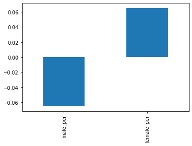
- Female_num correlates positively whereas male_num correlates negatively with Sat scores
- Racial inequality in sat scores can be identified easily from above (white_per, hispanic_per, black_per, asian_per)
Plotting stage
Now that we have prepared our data, drawn some insights from it as well. Let’s now do some exploratory charts and maps for a better understanding of the problem at hand
# Converting Latitude and Longitude to float values
full['Latitude'] = pd.to_numeric(full['Latitude'],errors='coerce')
full['Longitude'] = pd.to_numeric(full['Longitude'],errors='coerce')

schools_map = folium.Map(location=[full['Latitude'].mean(), full['Longitude'].mean()], zoom_start=10)
marker_cluster = plugins.MarkerCluster().add_to(schools_map)
for name, row in full.loc[~full['Latitude'].isnull()].iterrows():
    folium.Marker([row["Latitude"], row["Longitude"]], popup="{0}: {1}".format(row["dbn"], row["school_name"])).add_to(marker_cluster)
schools_map.save('schools.html')
schools_map
Let’s try plotting a heatmap to better visualize school density across NY
schools_heatmap = folium.Map(location=[full['Latitude'].mean(), full['Longitude'].mean()], zoom_start=10)
schools_heatmap.add_children(plugins.HeatMap([[row["Latitude"], row["Longitude"]] for name, row in full.loc[~full['Latitude'].isnull()].iterrows()]))
schools_heatmap.save("heatmap.html")
schools_heatmap
Interesting, Let’s try assessing further if there is any difference in SAT scores between the school districs
# Aggregating data at district level
district_data = full.groupby("school_dist").agg(np.mean)
district_data.reset_index(inplace=True)
district_data['school_dist'] = district_data['school_dist'].apply(lambda x: str(int(x)))
districts_geojson = pygeoj.load(filepath='districts.geojson')

# Defining a function to overlay heatmap distribution of a metric over the district maps
def show_district_map(col,dist):
    districts = folium.Map(location=[full['Latitude'].mean(), full['Longitude'].mean()], zoom_start=10)
    districts.choropleth(
    geo_data=dist,
    data=district_data,
    columns=['school_dist', col],
    key_on='feature.properties.school_dist',
    fill_color='YlGn',
    fill_opacity=0.7,
    line_opacity=0.2,
    )
    return districts

show_district_map("sat_score",districts_geojson).save("districts_sat.html")
show_district_map("sat_score",districts_geojson)
This looks great! Now that we have developed a basic understanding of the dataset and SAT score variation across districts. Let’s look further into the analysis angles that we had proposed earlier.
%matplotlib inline
full.plot.scatter(x='total_enrollment', y='sat_score')
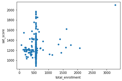
Hmm, There is not exactly a correlation here. Its just that there is a cluster of schools with low enrollment and low sat scores. Let’s try pulling up some names.
full.loc[(full['total_enrollment']<500)&(full['sat_score']<=1200),['name','sat_score']]
| name | sat_score | |
|---|---|---|
| 0 | HENRY STREET SCHOOL FOR INTERNATIONAL STUDIES | 1122.0 |
| 1 | UNIVERSITY NEIGHBORHOOD HIGH SCHOOL | 1172.0 |
| 3 | SATELLITE ACADEMY HS @ FORSYTHE STREET | 1174.0 |
| 9 | 47 THE AMERICAN SIGN LANGUAGE AND ENGLISH DUAL L | 1182.0 |
| 10 | FOOD AND FINANCE HIGH SCHOOL | 1194.0 |
| 11 | HIGH SCHOOL FOR HISTORY & COMMUNICATION | 1156.0 |
| 12 | HIGH SCHOOL OF HOSPITALITY MANAGEMENT | 1111.0 |
| 15 | THE FACING HISTORY SCHOOL | 1051.0 |
| 16 | THE URBAN ASSEMBLY ACADEMY OF GOVERNMENT AND LAW | 1148.0 |
| 17 | LOWER MANHATTAN ARTS ACADEMY | 1200.0 |
| 18 | THE JAMES BALDWIN SCHOOL: A SCHOOL FOR EXPEDITIO | 1188.0 |
| 19 | THE URBAN ASSEMBLY SCHOOL OF BUSINESS FOR YOUNG | 1127.0 |
| 20 | GRAMERCY ARTS HIGH SCHOOL | 1176.0 |
| 22 | EMMA LAZARUS HIGH SCHOOL | 1188.0 |
| 32 | LANDMARK HIGH SCHOOL | 1170.0 |
| 35 | LEGACY SCHOOL FOR INTEGRATED STUDIES | 1062.0 |
| 37 | BAYARD RUSTIN EDUCATIONAL COMPLEX | 1111.0 |
| 38 | VANGUARD HIGH SCHOOL | 1199.0 |
| 43 | UNITY CENTER FOR URBAN TECHNOLOGIES | 1070.0 |
| 49 | NEW DESIGN HIGH SCHOOL | 1168.0 |
| 50 | INDEPENDENCE HIGH SCHOOL | 1095.0 |
| 52 | LIBERTY HIGH SCHOOL ACADEMY FOR NEWCOMERS | 1156.0 |
| 56 | SATELLITE ACADEMY HIGH SCHOOL | 1032.0 |
After spending some time on Google to understand what is common between these schools, I have realized that most of these are schools where the minority enrollment and % of economically disadvantaged students is high. So its not actually low enrollment causing low sat scores but high % of minority students
full.plot.scatter(x='frl_percent', y='sat_score')
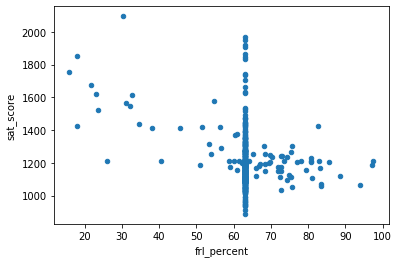
As expected, there is a negative correlation between FRL percent (indicative of % of minority & economically disadvantaged class) and sat scores. Higher the % of FRL in the school, lower is the sat score
full.plot.scatter(x='ell_percent', y='sat_score')
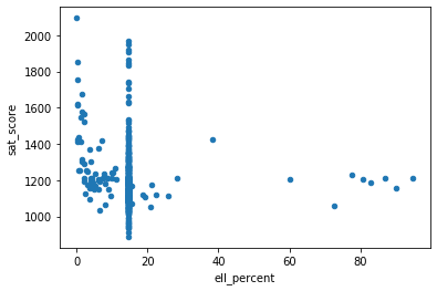
It looks like there are a group of schools with a high ell_percentage that also have low average SAT scores. We can investigate this at the district level, by figuring out the percentage of English language learners in each district, and seeing it if matches our map of SAT scores by district:
show_district_map('ell_percent',districts_geojson)
The distinction here is not very clear, probably due to the color palette chosen. We can for sure see that there is small district right in the middle which has very high ell_percent but not high sat scores.
Checking the correlation between survey responses and SAT Scores
full.corr()["sat_score"][["rr_s", "rr_t", "rr_p", "N_s", "N_t", "N_p", "saf_tot_11", "com_tot_11", "aca_tot_11", "eng_tot_11"]].plot.bar()
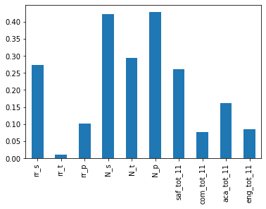
The only factors having a significant correlation with sat scores here are number of parents, students, and teachers responding to the survey, and the % of students responding to the survey. As these also correlate highly with total enrollment, it makes sense to say that schools with low frl percent, also have high survey response rates (that is not our concern at the moment though)
Exploring relationship between race and SAT scores
full.corr()["sat_score"][["white_per", "asian_per", "black_per", "hispanic_per"]].plot.bar()
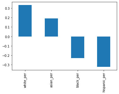
From above we can conclude that higher percentage of white and asian students lead to higher sat scores and the inverse holds true for black and hispanic students. It is likely that black and hispanic students are migrants who are also learning english language and are from economically disadvantaged community Let’s look at which schools have high white_per
full.plot.scatter(x='hispanic_per',y='sat_score')
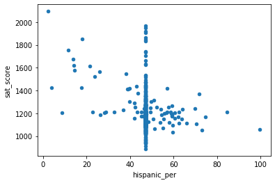
full.loc[(full['hispanic_per']<40)&(full['sat_score']>1400),['school_name','sat_score']]
| school_name | sat_score | |
|---|---|---|
| 6 | NEW EXPLORATIONS INTO SCIENCE TECHNO | 1621.0 |
| 8 | BARD HIGH SCHOOL EARLY COLLEGE | 1856.0 |
| 24 | INSTITUTE FOR COLLABORATIVE EDUCATION | 1424.0 |
| 25 | PROFESSIONAL PERFORMING ARTS HIGH SCH | 1522.0 |
| 26 | BARUCH COLLEGE CAMPUS HIGH SCHOOL | 1577.0 |
| 27 | N.Y.C. LAB SCHOOL FOR COLLABORATIVE S | 1677.0 |
| 28 | SCHOOL OF THE FUTURE HIGH SCHOOL | 1565.0 |
| 29 | N.Y.C. MUSEUM SCHOOL | 1419.0 |
| 30 | ELEANOR ROOSEVELT HIGH SCHOOL | 1758.0 |
| 31 | MILLENNIUM HIGH SCHOOL | 1614.0 |
| 41 | STUYVESANT HIGH SCHOOL | 2096.0 |
| 44 | TALENT UNLIMITED HIGH SCHOOL | 1416.0 |
| 51 | HIGH SCHOOL FOR DUAL LANGUAGE AND ASI | 1424.0 |
| 54 | HIGH SCHOOL M560 - CITY AS SCHOOL | 1415.0 |
| 55 | URBAN ACADEMY LABORATORY HIGH SCHOOL | 1547.0 |
These schools rank high in charts and host admission test and screening before admission, which is probably why hispanic_per ther is lower than others
Gender differences in SAT scores
full.corr()["sat_score"][["male_per", "female_per"]].plot.bar()
AP test scores & SAT scores
One last angle that we would be exploring here is the Advance Placement test and how it affects SAT scores. We already saw that number of AP test takers correlates strongly with SAT scores
full['ap_per'] = full['ap_test_takers_']/full['total_enrollment']
full.plot.scatter(x='ap_per',y='sat_score')
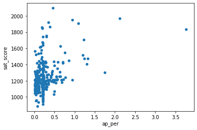
Let’s try pulling some names from the cluster in top right (excluding outliers) where sat_scores are high
full.loc[(full['ap_per']>0.3)&(full['sat_score']>1400),['school_name','sat_score']]
| school_name | sat_score | |
|---|---|---|
| 30 | ELEANOR ROOSEVELT HIGH SCHOOL | 1758.0 |
| 41 | STUYVESANT HIGH SCHOOL | 2096.0 |
| 55 | URBAN ACADEMY LABORATORY HIGH SCHOOL | 1547.0 |
| 74 | FIORELLO H. LAGUARDIA HIGH SCHOOL OF | 1707.0 |
| 81 | MANHATTAN CENTER FOR SCIENCE AND MATH | 1430.0 |
| 175 | NaN | 1969.0 |
| 182 | NaN | 1920.0 |
| 220 | NaN | 1833.0 |
| 275 | NaN | 1436.0 |
| 313 | NaN | 1431.0 |
| 320 | NaN | 1473.0 |
| 323 | NaN | 1627.0 |
| 351 | NaN | 1910.0 |
| 355 | NaN | 1514.0 |
| 356 | NaN | 1474.0 |
| 358 | NaN | 1449.0 |
| 374 | NaN | 1407.0 |
| 379 | NaN | 1868.0 |
| 405 | NaN | 1418.0 |
| 409 | NaN | 1953.0 |
Some Google searching reveals that these are mostly highly selective schools where you need to take a test to get in. It makes sense that these schools would have high proportions of AP test takers.
THE END!
This is all that we are going to cover as part of this project. I would like to thank DataQuest.io for guiding me through the project.